Digesting Data from NGINX Access Logs#
This notebook was created as an exercise in data manipulation and visualization in Python. The data used in this notebook consists of the last two months of searches on GitHub Search, as recorded in the NGINX access logs. The raw logs were parsed and enriched with geographical data, which was retrieved from ipinfo. Our end-goal is to gain more insight into the usage of the aforementioned platform. Before we begin, we need to import all the necessary library utilities.
from ast import literal_eval

from IPython.display import Markdown
from geopandas import read_file
from geopandas.datasets import get_path
from matplotlib.pyplot import bar, figure, pie, show, subplot
from pandas import DataFrame
from pandas import concat, json_normalize, read_csv
from shapely.geometry import Point


figsize = (20, 10)

def summarize(data_frame: DataFrame):
    index = ["count", "mean", "min", "max"]
    data = [data_frame.count(), data_frame.mean(), data_frame.min(), data_frame.max()]
    return DataFrame(data, index=index)

def get_top_n(data_frame: DataFrame, n: int = 10):
    data_frame_counts = data_frame.value_counts()
    data_frame_top = data_frame_counts.head(n - 1)
    data_frame_other_count = data_frame_counts.tail(1 - n).sum()
    data_frame_other = DataFrame(data={"count": [data_frame_other_count]}, index=["Other"])
    return concat([data_frame_top, data_frame_other])
With that out of the way, we can now read the CSV file, and convert the string representation of the JSON data into Python dictionaries.
columns = ["access", "city"]
converters = { key: literal_eval for key in columns }
df = read_csv("access.csv", header=None, names=columns, converters=converters)
df.head()
| access | city | |
|---|---|---|
| 0 | {'ip': '174.2.241.68', 'time': '2023-12-19T00:... | {'name': 'Saskatoon', 'region': 'Saskatchewan'... |
| 1 | {'ip': '174.2.241.68', 'time': '2023-12-19T00:... | {'name': 'Saskatoon', 'region': 'Saskatchewan'... |
| 2 | {'ip': '174.2.241.68', 'time': '2023-12-19T00:... | {'name': 'Saskatoon', 'region': 'Saskatchewan'... |
| 3 | {'ip': '140.205.11.7', 'time': '2023-12-19T01:... | {'name': 'Hangzhou', 'region': 'Zhejiang', 'co... |
| 4 | {'ip': '140.205.11.7', 'time': '2023-12-19T02:... | {'name': 'Hangzhou', 'region': 'Zhejiang', 'co... |
Next, let’s transform our two-column DataFrame into a single DataFrame with the JSON data expanded into columns. Let’s start with the city column:
mappings = {
  "name": "city",
  "country_continent_name": "continent_name",
  "country_continent_code": "continent_code",
  "position_latitude": "latitude",
  "position_longitude": "longitude",
}
city = json_normalize(df.city, sep="_").rename(columns=mappings)
coordinate_mapper = lambda row: Point(row.longitude, row.latitude)
city["coordinates"] = city.apply(coordinate_mapper, axis=1)
city.drop(columns=["latitude", "longitude"], inplace=True)
city = city[["city", "region", "country_name", "country_code", "continent_name", "continent_code", "coordinates"]]
city.head()
| city | region | country_name | country_code | continent_name | continent_code | coordinates | |
|---|---|---|---|---|---|---|---|
| 0 | Saskatoon | Saskatchewan | Canada | CA | North America | NA | POINT (-106.6689 52.1324) |
| 1 | Saskatoon | Saskatchewan | Canada | CA | North America | NA | POINT (-106.6689 52.1324) |
| 2 | Saskatoon | Saskatchewan | Canada | CA | North America | NA | POINT (-106.6689 52.1324) |
| 3 | Hangzhou | Zhejiang | China | CN | Asia | AS | POINT (120.1614 30.2936) |
| 4 | Hangzhou | Zhejiang | China | CN | Asia | AS | POINT (120.1614 30.2936) |
Let’s do the same for the access column:
access = json_normalize(df.access, sep="_", max_level=0)
access = access.join(json_normalize(access["user_agent"], sep="_"))
access.drop(columns=["user_agent"], inplace=True)
access = access[["ip", "time", "query", "status", "size", "browser", "os", "device", "referer"]]
access.head()
| ip | time | query | status | size | browser | os | device | referer | |
|---|---|---|---|---|---|---|---|---|---|
| 0 | 174.2.241.68 | 2023-12-19T00:02:05Z | {'nameEquals': ['false'], 'language': ['c++'],... | 200 | 71.78 KB | Chrome 120.0.0 | Mac OS X 10.15.7 | PC | https://seart-ghs.si.usi.ch/ |
| 1 | 174.2.241.68 | 2023-12-19T00:54:17Z | {'nameEquals': ['false'], 'language': ['c++'],... | 200 | 62 bytes | Chrome 120.0.0 | Mac OS X 10.15.7 | PC | https://seart-ghs.si.usi.ch/ |
| 2 | 174.2.241.68 | 2023-12-19T00:54:38Z | {'name': ['purpose'], 'nameEquals': ['false'],... | 200 | 62 bytes | Chrome 120.0.0 | Mac OS X 10.15.7 | PC | https://seart-ghs.si.usi.ch/ |
| 3 | 140.205.11.7 | 2023-12-19T01:58:11Z | {'nameEquals': ['false'], 'topic': ['react'], ... | 200 | 47.42 KB | Chrome 119.0.0 | Mac OS X 10.15.7 | PC | https://seart-ghs.si.usi.ch/ |
| 4 | 140.205.11.7 | 2023-12-19T02:00:47Z | {'name': ['react'], 'nameEquals': ['false'], '... | 200 | 26 KB | Chrome 119.0.0 | Mac OS X 10.15.7 | PC | https://seart-ghs.si.usi.ch/ |
Merging the two together:
df = DataFrame.join(access, city)
df.head()
| ip | time | query | status | size | browser | os | device | referer | city | region | country_name | country_code | continent_name | continent_code | coordinates | |
|---|---|---|---|---|---|---|---|---|---|---|---|---|---|---|---|---|
| 0 | 174.2.241.68 | 2023-12-19T00:02:05Z | {'nameEquals': ['false'], 'language': ['c++'],... | 200 | 71.78 KB | Chrome 120.0.0 | Mac OS X 10.15.7 | PC | https://seart-ghs.si.usi.ch/ | Saskatoon | Saskatchewan | Canada | CA | North America | NA | POINT (-106.6689 52.1324) |
| 1 | 174.2.241.68 | 2023-12-19T00:54:17Z | {'nameEquals': ['false'], 'language': ['c++'],... | 200 | 62 bytes | Chrome 120.0.0 | Mac OS X 10.15.7 | PC | https://seart-ghs.si.usi.ch/ | Saskatoon | Saskatchewan | Canada | CA | North America | NA | POINT (-106.6689 52.1324) |
| 2 | 174.2.241.68 | 2023-12-19T00:54:38Z | {'name': ['purpose'], 'nameEquals': ['false'],... | 200 | 62 bytes | Chrome 120.0.0 | Mac OS X 10.15.7 | PC | https://seart-ghs.si.usi.ch/ | Saskatoon | Saskatchewan | Canada | CA | North America | NA | POINT (-106.6689 52.1324) |
| 3 | 140.205.11.7 | 2023-12-19T01:58:11Z | {'nameEquals': ['false'], 'topic': ['react'], ... | 200 | 47.42 KB | Chrome 119.0.0 | Mac OS X 10.15.7 | PC | https://seart-ghs.si.usi.ch/ | Hangzhou | Zhejiang | China | CN | Asia | AS | POINT (120.1614 30.2936) |
| 4 | 140.205.11.7 | 2023-12-19T02:00:47Z | {'name': ['react'], 'nameEquals': ['false'], '... | 200 | 26 KB | Chrome 119.0.0 | Mac OS X 10.15.7 | PC | https://seart-ghs.si.usi.ch/ | Hangzhou | Zhejiang | China | CN | Asia | AS | POINT (120.1614 30.2936) |
We can now initiate our analysis. Let’s start off easy by calculating the total number of searches per day:
date_only = lambda ts: ts.split("T")[0]
days_accessed = df.time.map(date_only)
daily_visitors = days_accessed.value_counts().sort_index()
daily_visitors.plot(figsize=figsize)
<Axes: xlabel='time'>
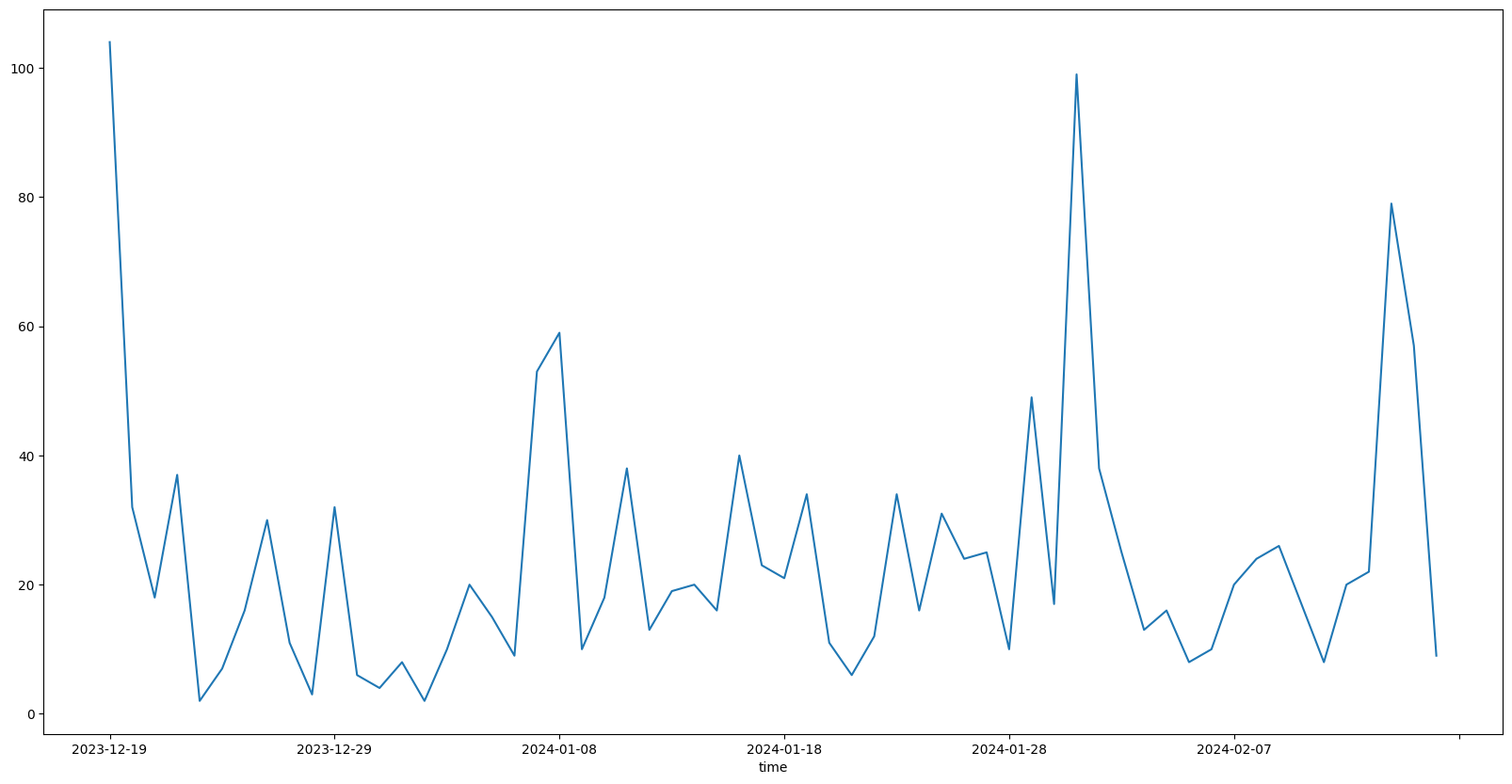
Seems like the platform has been accessed every day. Let’s break this 60-day period down into a statistical summary:
summarize(daily_visitors.to_frame())
| count | |
|---|---|
| count | 60.000000 |
| mean | 24.266667 |
| min | 2.000000 |
| max | 104.000000 |
As we can see, the average number of daily searches is around 25, with the minimum being as low as only 2 searches in a day, and the maximum being more than 100 searches in a single day! Keep in mind that we are looking at the total number of searches conducted by any user on a daily basis. This means that the number of unique visitors is likely to be lower. Let’s calculate that next:
ip_access = df[['time', 'ip']]
ip_access.loc[:, "time"] = ip_access.loc[:, "time"].map(date_only)
ip_access_by_day = ip_access.groupby("time").nunique()
ip_access_by_day.plot(figsize=figsize)
<Axes: xlabel='time'>

And on average:
summarize(ip_access_by_day)
| ip | |
|---|---|
| count | 60.000000 |
| mean | 7.766667 |
| min | 1.000000 |
| max | 21.000000 |
Having gathered insights on daily traffic, we can now move on calculating the distribution of traffic by continent and country.
continent_top = get_top_n(df.continent_name, 5)
country_top = get_top_n(df.country_name)

autopct = "%1.1f%%"
figure(figsize=figsize)
subplot(1, 2, 1)
pie(list(continent_top["count"]), labels=continent_top.index, autopct=autopct)
subplot(1, 2, 2)
pie(list(country_top["count"]), labels=country_top.index, autopct=autopct)
show()
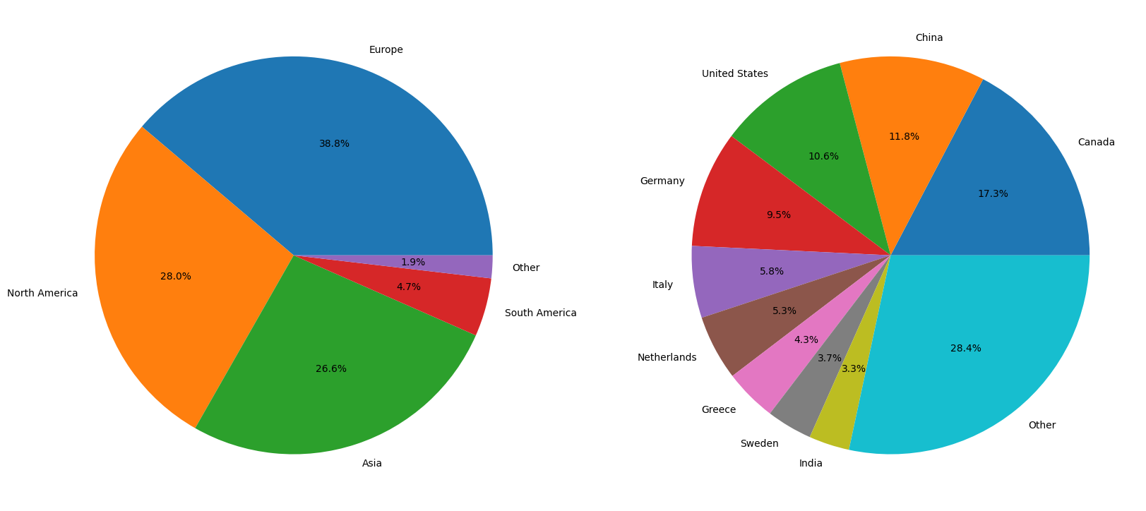
While the distribution of traffic by continent is relatively balanced and simple to comprehend, the distribution of traffic by country appears to be more complex. More than a quarter of the traffic is widely distributed across a large number of countries. For this reason, plotting the data on a map might be more insightful. To do that, we must first load some geographical geometry data:
country_geometry = read_file(get_path("naturalearth_lowres"))
country_geometry = country_geometry[country_geometry.continent != "Antarctica"]
country_geometry = country_geometry[country_geometry.pop_est > 0]
country_geometry = country_geometry[["name", "geometry"]]
country_geometry.rename(columns={"name": "country_name"}, inplace=True)
country_geometry.set_index("country_name", inplace=True)
country_geometry.rename(index={"United States of America": "United States"}, inplace=True)
country_geometry
/tmp/ipykernel_1780/2322404391.py:1: FutureWarning: The geopandas.dataset module is deprecated and will be removed in GeoPandas 1.0. You can get the original 'naturalearth_lowres' data from https://www.naturalearthdata.com/downloads/110m-cultural-vectors/.
  country_geometry = read_file(get_path("naturalearth_lowres"))
| geometry | |
|---|---|
| country_name | |
| Fiji | MULTIPOLYGON (((180.00000 -16.06713, 180.00000... |
| Tanzania | POLYGON ((33.90371 -0.95000, 34.07262 -1.05982... |
| W. Sahara | POLYGON ((-8.66559 27.65643, -8.66512 27.58948... |
| Canada | MULTIPOLYGON (((-122.84000 49.00000, -122.9742... |
| United States | MULTIPOLYGON (((-122.84000 49.00000, -120.0000... |
| ... | ... |
| Serbia | POLYGON ((18.82982 45.90887, 18.82984 45.90888... |
| Montenegro | POLYGON ((20.07070 42.58863, 19.80161 42.50009... |
| Kosovo | POLYGON ((20.59025 41.85541, 20.52295 42.21787... |
| Trinidad and Tobago | POLYGON ((-61.68000 10.76000, -61.10500 10.890... |
| S. Sudan | POLYGON ((30.83385 3.50917, 29.95350 4.17370, ... |
176 rows × 1 columns
We can now plot our location data on a world map:
country_count = df.country_name.value_counts()
world_count = country_geometry.join(country_count)
world_count.plot(
  figsize=figsize,
  column="count",
  cmap="viridis",
  legend=True,
  missing_kwds={
    "color": "lightgrey",
    "label": "No Data",
    "edgecolor": "red",
  },
  legend_kwds={
    "label": "Traffic",
    "shrink": 0.65,
  },
)
<Axes: >

From this we can not only see all the countries that the platform has been accessed from, but also the countries that it has not been accessed from. What’s interesting, small amounts of traffic were recorded in Africa (Morocco and Egypt), as well as South America (Brazil and Chile).
Shifting our focus to a different angle, we can now analyze the distribution of traffic by browser, operating system, and device. To start, let’s first isolate the relevant columns into a smaller DataFrame:
user_agent = df[["browser", "os"]]
user_agent
| browser | os | |
|---|---|---|
| 0 | Chrome 120.0.0 | Mac OS X 10.15.7 |
| 1 | Chrome 120.0.0 | Mac OS X 10.15.7 |
| 2 | Chrome 120.0.0 | Mac OS X 10.15.7 |
| 3 | Chrome 119.0.0 | Mac OS X 10.15.7 |
| 4 | Chrome 119.0.0 | Mac OS X 10.15.7 |
| ... | ... | ... |
| 1451 | Chrome 121.0.0 | Windows 10 |
| 1452 | Chrome 121.0.0 | Windows 10 |
| 1453 | Chrome 121.0.0 | Windows 10 |
| 1454 | Firefox 122.0 | Windows 10 |
| 1455 | Firefox 122.0 | Windows 10 |
1456 rows × 2 columns
Notice that both browser and os contain versioning information, which may potentially lead to more numerous unique values. To group the values within their respective families, we can apply a simple transformation:
strip_version = lambda x: x.rsplit(' ', 1)[0]
user_agent = user_agent.map(strip_version)
user_agent
| browser | os | |
|---|---|---|
| 0 | Chrome | Mac OS X |
| 1 | Chrome | Mac OS X |
| 2 | Chrome | Mac OS X |
| 3 | Chrome | Mac OS X |
| 4 | Chrome | Mac OS X |
| ... | ... | ... |
| 1451 | Chrome | Windows |
| 1452 | Chrome | Windows |
| 1453 | Chrome | Windows |
| 1454 | Firefox | Windows |
| 1455 | Firefox | Windows |
1456 rows × 2 columns
With the data in a more manageable state, we can now calculate the distribution of traffic by browser and operating system:
browsers_top = get_top_n(user_agent.browser, 5)
operating_systems_top = get_top_n(user_agent.os, 5)

figure(figsize=figsize)
subplot(1, 2, 1)
bar(browsers_top.index, browsers_top["count"])
subplot(1, 2, 2)
bar(operating_systems_top.index, operating_systems_top["count"])
show()
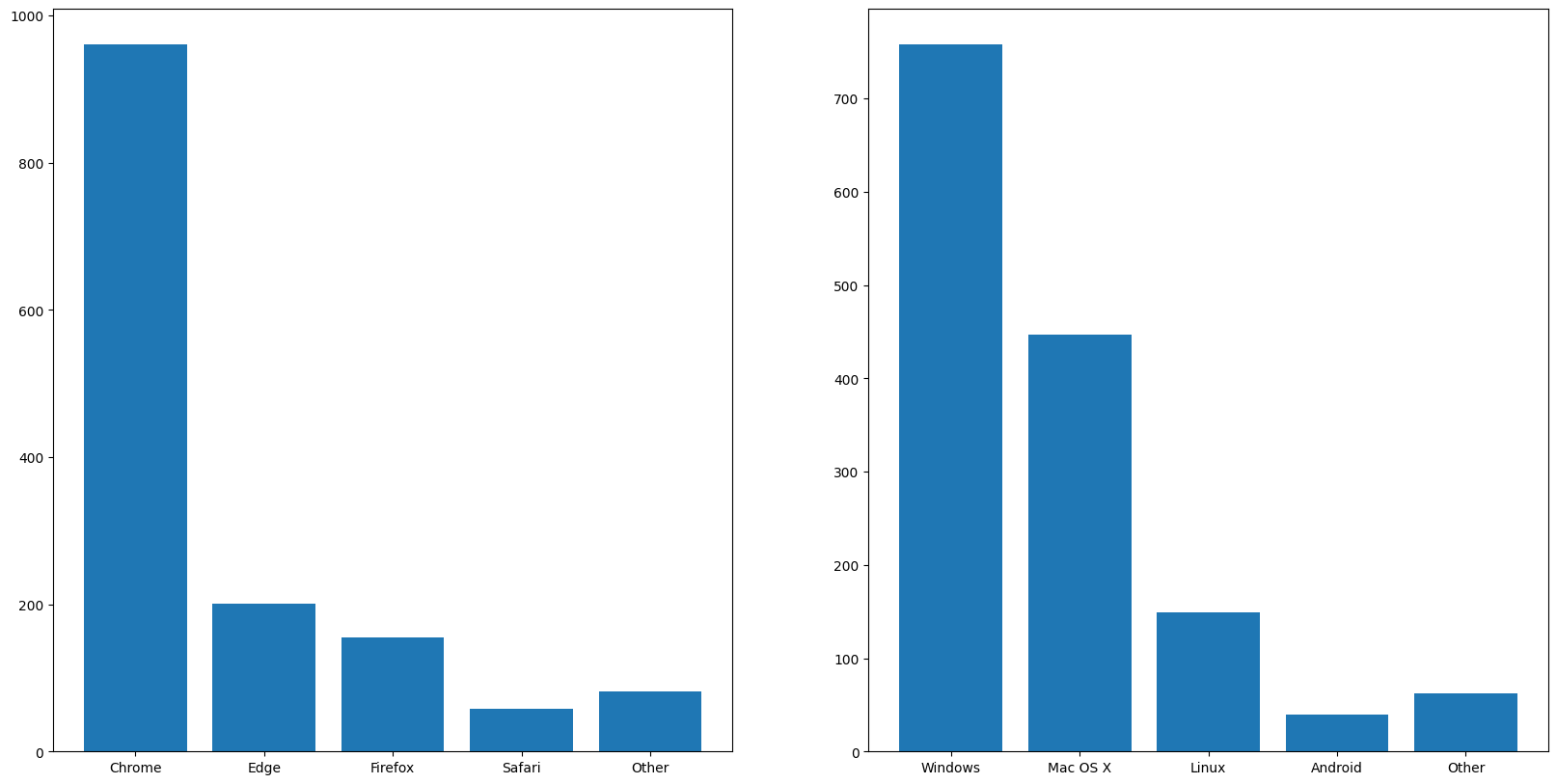
To no one’s surprise, Chrome reigns supreme in the browser market, closely followed by Edge and Firefox. Although we develop and test our platform UI exclusively on Chrome, the fact that other browsers are used puts an emphasis on the need for cross-browser compatibility, which would be ensured through end-to-end testing. While manual testing would be too time-consuming, automated testing would be a more efficient solution. Although you might be asking yourself why we are considering operating systems for a web application, the answer lies in the fact that the platform is also accessible through mobile devices. As such, we made sure that the design of the site was responsive. While the data shows that a minute fraction of the traffic comes from mobile devices, it’s important to keep in mind that a good first impression from a handheld can convince users to try the desktop version as well.
To conclude our analysis, let’s take a look at what users are searching for, starting with the most popular query parameters. Note that for this analysis, we will not consider:
pageandper_page, as they are used for paginationnameEquals, as it is always included in the query
Furthermore, the ranged parameters (e.g. starsMin and starsMax) will be grouped under a single umbrella (i.e. stars).
blacklist = ["page", "per_page", "nameEquals"]
query_keys = lambda query: query.keys()
query_parameters = df["query"].map(query_keys)
query_parameters_by_query = query_parameters.explode()
query_parameters_by_query = query_parameters_by_query.loc[~query_parameters_by_query.isin(blacklist)]
query_parameters_by_query = query_parameters_by_query.str.removesuffix("Min")
query_parameters_by_query = query_parameters_by_query.str.removesuffix("Max")
query_parameters_by_query_count = query_parameters_by_query.value_counts()
query_parameters_by_query_count.plot.bar(figsize=figsize)
<Axes: xlabel='query'>
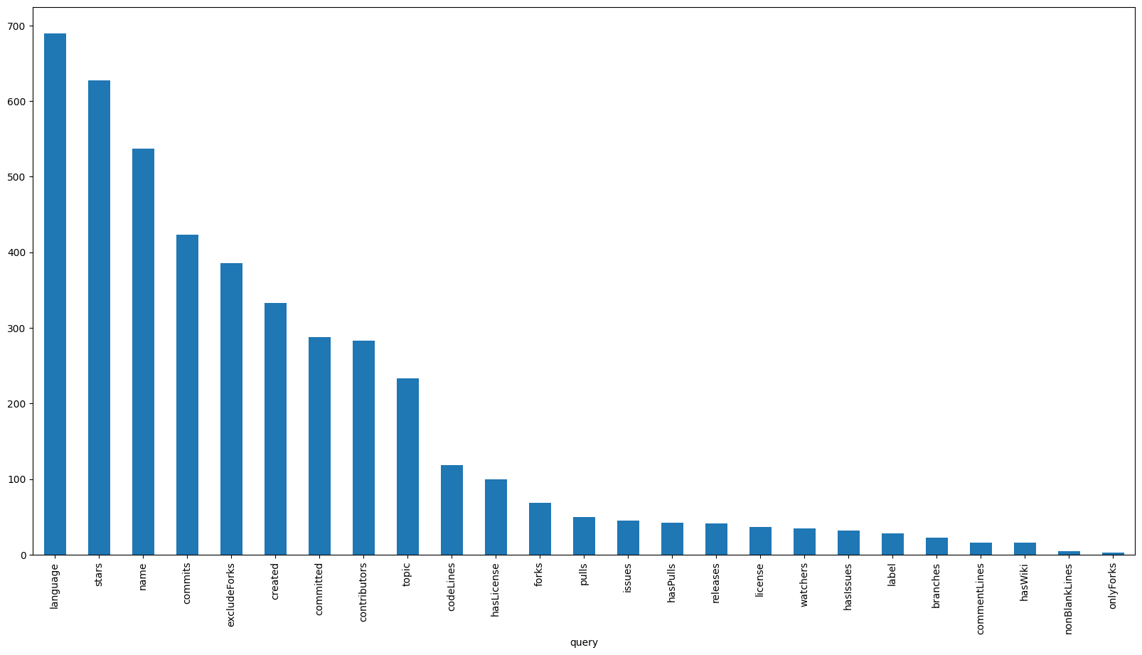
To no particular surprise, we can see that language comes out on top, followed closely by stars, name and commits. What is interesting however is that the topic parameter placed in the top 10, in spite of being a relatively new addition to the dataset. This could be an indication that the feature is being well received by the users. On the flipside, exact match parameters such as label and license have seen significantly less use. This is most likely due to the fact that there is currently no way to specify multiple values for a single query, which in my humble opinion is a feature we should consider prioritizing in the future.
Given that the language parameter is the most popular, it would be interesting to see which languages users search for the most. To do this, we can extract the language parameter values and calculate their distribution:
def get_languages(query: dict):
  if "language" in query:
    first, = query["language"]
    return first.lower()
  return None

query_parameter_language = df["query"].map(get_languages).dropna()
query_parameter_language_count = get_top_n(query_parameter_language, 4)
figure(figsize=figsize)
pie(query_parameter_language_count["count"], labels=query_parameter_language_count.index, autopct=autopct)
show()

As was expected, Java, Python and JavaScript, the three of the most popular programming languages in the world constitute a cumulative 70% of language-specific searches. While looking at the top does not reveal anything particularly surprising, it’s at the very bottom where some new insights are obtained:
least_popular_languages = query_parameter_language.value_counts().tail()
least_popular_languages_names = list(least_popular_languages.keys())
Markdown("\n".join([f"- {item}" for item in least_popular_languages_names]))
dart, kotlin
haskell
c/c++
npm
lua
The first thing that stands out is the fact that Lua and Haskell were both queried. Although we do not mine these languages, it’s worth considering adding them to the list of future targets. The second thing that stands out is the fact that dart, kotlin and c/c++ were search terms. Echoing the sentiment from the previous section, it’s worth considering adding the ability to search for multiple languages at once, allowing sampling on a set of languages.